Anyway, the big news today is definitely Brexit, with a narrow majority of Brits voting to leave the EU. I don't know what to say about this, as Mexico isn't, and never has been, in a similar situation. From what I see on social media--particularly Twitter--people who voted to leave the EU are labeled de facto bigots, whereas people who voted to remain are branded as corrupt, self-hating authoritarians. What seems to be unambiguous is the dismay of the scientific community at the situation. The impact around the world will play out slowly over the next few months, but already there are warnings from experts of future financial and, potentially, political turmoil. For now, Mexican technocrats have used Brexit as an excuse to pass budgetary cuts--no one believes them, as always, and they go ahead anyway, as always.
Speaking of Mexico, the news out of the southern state of Oaxaca made headlines around the world and, as is usually the case anytime Mexico is noticed internationally, it was bad news. Teachers protested last weekend over an education reform that was passed a couple of years ago and has been phased into practice since. The crux of the issue is that the government insists that teachers need to be evaluated, but the teachers insist that the evaluation methods are extremely unfair and hurt teachers in poorer states and neighborhoods the most. Last Sunday, teachers protested and were met by riot police that had been waiting for them. The riot police were accompanied by hundreds of armed federal agents. Nobody knows who started the violence, but eventually shots were fired and eight people died; over a hundred more were wounded. Each side accuses the other of starting the violence, and there is no clear path forward at the time. Oaxaca is one of the poorest states in Mexico, and the teacher's union (known as the CNTE) is particularly strong there; there are frequent protests, especially around the month of May, when teacher's day is celebrated in Mexico. The CNTE union is known for its massive national mobilizations and month-long strikes in Oaxaca, and the educational reform has made them more upset than usual--rightly so, I think.
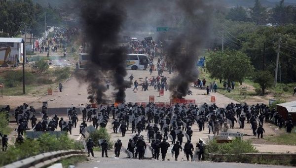 |
| Federal agents in riot gear confront protesters in Oaxaca, Mexico. |
* * *
Anyway, on the Physics side of things, I had a modestly productive week. I'm working my way through Carroll's text, Spacetime and Geometry, specifically the third chapter on curvature. As a backup, I went back to the book by Schutz, which is a couple notches below Carroll's in difficulty and has many, more 'basic' exercises. Curvature is a big deal in General Relativity, since gravity is understood as an effect of geometry rather than a force. We're all familiar with curved surfaces and objects, such as basketballs and the Earth's surface; the idea in GR is that spacetime is curved, and what we perceive as gravity is the manifestation of that curvature.
More specifically, on curved, continuous surfaces (known technically as manifolds) one has to account for the way coordinates are bent and twisted along with the surface. Up/down, left/right, forward/backward, and past/future point in different directions depending on where one is, and how one is moving. Specifying coordinates and higher concepts such as velocities or trajectories is much harder than in the regular, flat geometry we all are used to. It is necessary, then, to introduce geometrical concepts that are much more general than those of Euclidean (i.e., flat) geometry, and to generalize calculus accordingly as well. As an example, the derivative for a vector looks like this in generalized curved coordinates: \[\frac{\partial \vec{V}}{\partial x^\beta} = \frac{\partial V^\alpha}{\partial x^\beta }\vec{e}_{\alpha}+\frac{\partial \vec{e}_\alpha}{\partial x^\beta }V^\alpha.\] In flat cartesian coordinates the second term is always zero, since the basis vectors \( \vec{e}_\alpha\) are constant (they're just unit vectors always pointing in the \(x\), \(y\), and \(z\) directions) and their derivative is zero. But in general curvilinear coordinates, the basis vectors change along a path; they get twisted, turned, or stretched on different parts of the surface. In general, these changes that the basis vectors undergo (the term \(\frac{\partial \vec{e}_\alpha}{\partial x^\beta }\) above) can be written as a linear combination of some coefficients that act upon the basis vectors. These coefficients can be written as mathematical gizmos that look like this: \[ \frac{\partial \vec{e}_\alpha}{\partial x^\beta } = \Gamma^{\mu}_{\,\,\,\alpha \beta} \vec{e}_\mu.\] These gizmos are known as Christoffel symbols, and what they do is adjust for how the basis vectors \(\vec{e}_\mu\) change along the curvature of the surface. So, for the above vector \(\vec(V)\), the derivative can now be written as \[\frac{\partial \vec{V}}{\partial x^\beta} = \left( \frac{\partial V^\alpha}{\partial x^\beta }+V^\mu\,\Gamma^{\alpha}_{\,\,\,\mu\beta} \right )\vec{e}_{\alpha}.\]
Armed with these gizmos, we can generalize ordinary vector calculus operations to curved space. The problem is where to get them in the first place! Luckily, they can be calculated from the metric of the manifold: this is the one defining characteristic for the manifold's curved character, and is usually written in the form of an equation for what the line element (a typical, small line that lives in the manifold) looks like. The line element for the surface of a sphere, for example, is fairly dull: \[ ds^2 = r^2\,d\theta^2 + r^2 \sin^2\theta \, d\phi^2.\] (Notice we only need to specify two angles, latitude and longitude, to move along the surface of the sphere; once you live on a sphere and are confined to move along it's surface, the radius is not much use, that's why there's no \(dr^2\) term.) Once we have the equation for the metric, and after we write it in matrix form \(g\), we can calculate the coefficients according to \[ \Gamma^{\gamma}_{\,\,\,\beta \alpha} = \frac{1}{2}g^{\alpha \gamma} \left( \partial_\mu g_{\alpha\beta} + \partial_\beta g_{\alpha\mu} - \partial_\alpha g_{\beta\mu} \right).\]
Obviously I've glossed over a lot of things, pulled things from under my sleeve, and generally omitted lots of details. Eventually I'll explain these things in much grater detail and include pictures for these things so it'll become clearer what it is I'm talking about, but I have to learn to use the tikz and pgfplots \(LaTeX\) packages properly, which takes some time. Anyway, if all goes well, I'll have something to write about next week at the latest.
No comments:
Post a Comment